Effective Variational Learning with IVON on GPT-2

Bayesian methods are considered impractical at large scale, and even when we are able to make them work for large deep networks (say using approximations), we don’t expect them to match the performance of optimizers such as SGD or Adam. In our recent work, we present results against this belief and show effectiveness of variational learning (called IVON) for large deep networks such as GPT-2, obtaining consistent improvement over AdamW with nearly identical runtime. These results are significant because they are obtained by directly optimizing the variational (Bayesian) objective. This is unlike methods like MC-dropout or SWAG which do not directly optimize such objectives, even though they have variational interpretations. In this blog, I describe some major point of the paper.

1. Main results and the IVON algorithm
2. Using IVON as a drop-in replacement of AdamW
3. Results on OOD detection, model merging in LLMs, and model understanding
4. A brief history of how we got here.

For practitioners, who are interested in using IVON, just reading Item 2 is sufficient to get started.

Paper: Variational Learning is Effective for Large Deep Networks
Code: https://github.com/team-approx-bayes/ivon

MAIN RESULTS

The most exciting result is for GPT-2. We ran IVON on OpenWebText data (49.2 billion tokens) to fit three GPT-2 models with parameters sizes of 773M, 355M, and 125M respectively. These are quite large data and models but IVON closely follows the trajectory of AdamW with a slightly better performance in the end to get around 0.2-0.4 decrease in perplexity. Some NLP researchers tell me this is significant and I believe them.

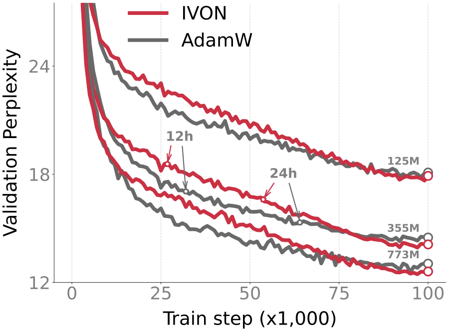
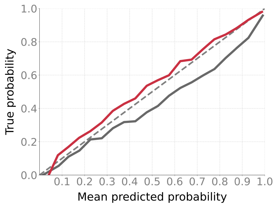
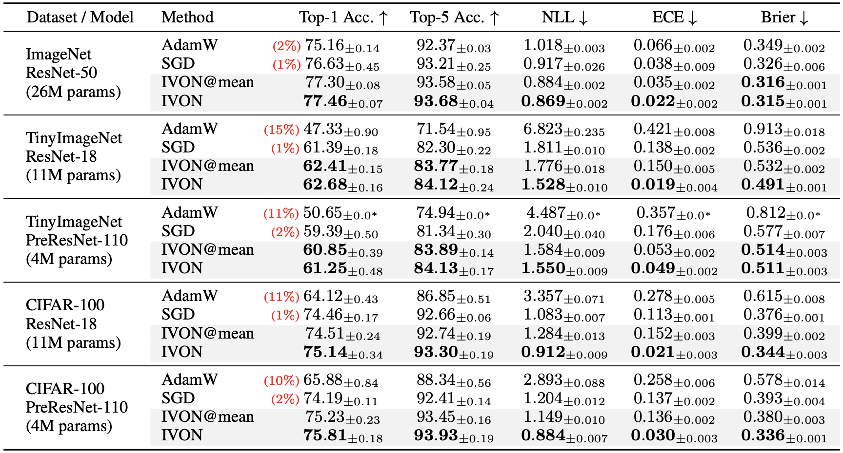
For GPT-2, IVON’s slightly lagging behind AdamW in terms of runtime which is due to posterior sampling (more on this later). However, the overhead due to sampling is worth it because it makes IVON’s weight-uncertainty (that is, variance estimates of the weights) much better than AdamW. For instance, on ImageNet, IVON not only gets better accuracy than both AdamW and SGD (around 1-2% in the first figure) but its predictions are also better calibrated (the red line is closer to the diagonal in the second figure). The cost of posterior sampling is negligible at ImageNet scale and the runtime of IVON is almost identical to AdamW.

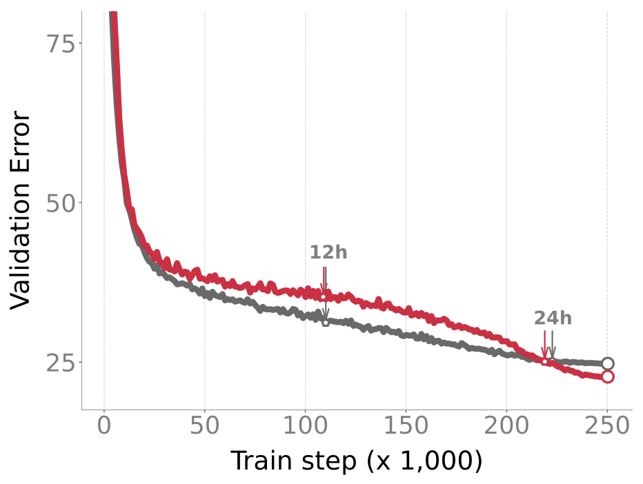
An advantage of posterior sampling is that, unlike AdamW, IVON does not suffer from overfitting. It is well-known for image classification that AdamW, when run for a long time without early stopping, starts to overfit. It also consistently underperforms compared to SGD. IVON does not have this problem and we see consistent improvement over SGD and no overfitting like AdamW.

There are additional benefits of IVON, some of which I will describe later (see OOD detection and second-order information). These include

1. better predictive uncertainty than alternatives, such as, MC-dropout and SWAG.
2. its use for finetuning LLMs and to reduce the cost of model-merging.
3. faithful prediction of generalization for diagnostics and early stopping.
4. its use for understanding sensitivity to data which is often challenging at large-scale due to ill-conditioning.

Before these, let me briefly describe the IVON algorithm first.

THE IVON ALGORITHM

The IVON algorithm is derived using the Bayesian Learning rule of Khan and Rue and finds a Gaussian posterior-approximation over network weights by optimizing a variational (Bayesian) objective. The easiest way to understand IVON by directly comparing it to Adam or RMSprop, as shown in this (not so precise) pseudo-code where the differences are highlighted in red.

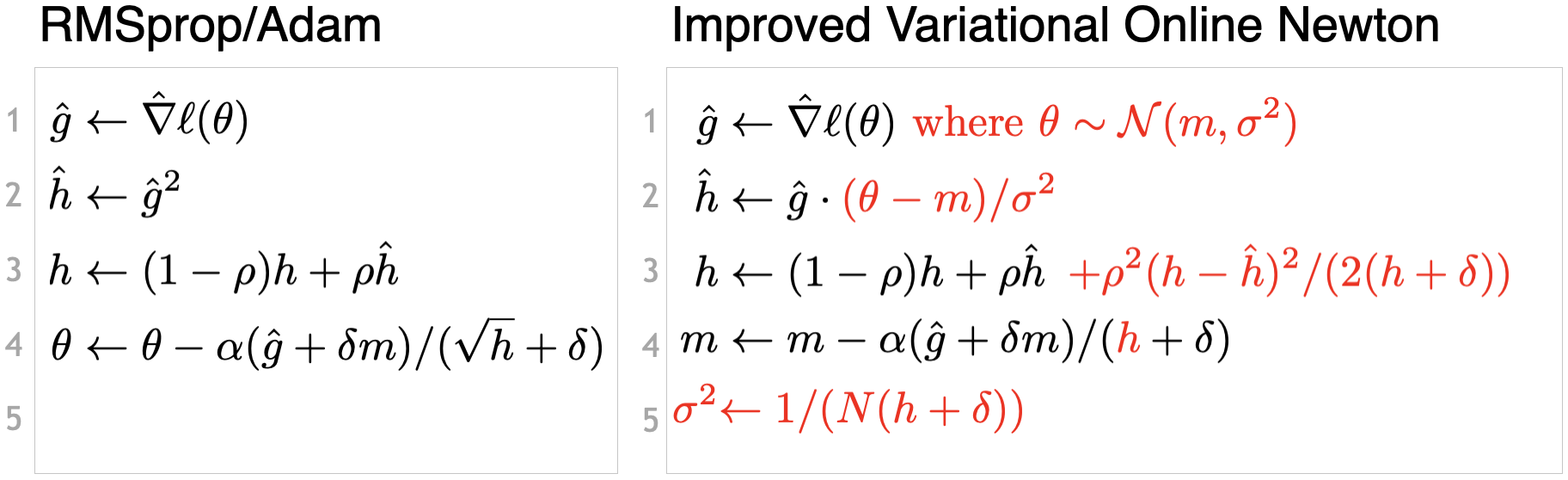
There are the following differences:

1. Unlike Adam, which returns one vector $\theta$, IVON returns two vectors: the mean $m$ and variance $\sigma^2$; see line 4-5. The mean $m$ plays the same role as $\theta$ in Adam to perform predictions. The variance vector $\sigma$ provides an uncertainty/confidence estimate: larger entries imply that the corresponding entries in $m$ can change a lot, for example, when data of training conditions are perturbed.
2. To estimate $\sigma$ faithfully, IVON perturbs the location where gradients are computed. This is done in line 1 where $\theta$ is sampled from a Gaussian. This is where the additional cost in IVON comes from, but it is crucial to get better $\sigma$.
3. Instead of using square of minibatch gradient $\hat{g}^2$, IVON computes a Monte-Carlo estimate of the Hessian. This is shown in line 2 where $\hat{g}$ is multiplied by $(\theta-m)/\sigma^2$. This is simply the reparameterization trick and gives an unbiased estimate of the Hessian. You can think of this as a perturbation to $\hat{g}$ to get an idea of the curvature; the perturbation $(\theta-m)/\sigma$ can also be seen as a sample from a standard Gaussian. Unlike Adam, IVON estimates an unbiased estimate of second-order information, which is subsequently used to compute $\sigma$ (in line 5)
4. In line 3, a correction term is added to ensure that the learning-rate adaptation vector $h$ is never negative. The cost of this step is minor but it improves stability of IVON by avoiding negative Hessians for nonconvex problems. The correction is derived using Riemannian gradient descent in the original work of Lin et al. 2020, but I will not go into details here. This step is not needed if we find $h$ never becomes negative in practice.
5. Finally, line 4 is almost identical to Adam but there is no square-root over $h$. Unlike Adam, IVON takes a Newton-like step.

A detailed pseudo-code containing momentum and debiasing steps is given in the paper.

HOW TO USE IVON

Due to its similarity to RMSprop/Adam, IVON can be used as a direct drop-in replacement for them. In PyTorch, we simply need to add the following highlighted lines to switch from Adam to IVON.

import torch
+import ivon

train_loader = torch.utils.data.DataLoader(train_dataset) 
test_loader = torch.utils.data.DataLoader(test_dataset) 
model = MLP()

-optimizer = torch.optim.Adam(model.parameters())
+optimizer = ivon.IVON(model.parameters())

for X, y in train_loader:
+  for _ in range(train_samples):
+    with optimizer.sampled_params(train=True)
        optimizer.zero_grad()
        logit = model(X)
        loss = torch.nn.CrossEntropyLoss(logit, y)
        loss.backward()

  optimizer.step()

The code is easily modifiable to include multiple GPUs, multiple MC samples, and also gradient and Hessian accumulation steps. We provide an implementation of IVON as a PyTorch optimizer. Many practical tricks are discussed in the paper which are essential to make IVON work at large scale. To state them briefly: we set the $\delta$ parameter to values commonly used in Adam; no debiasing for $h$ is used; we never initialize $h$ to 0; we clip the gradients; we use similar learning rate schedule to Adam, etc. A useful hack is to make learning rate for $h$ very close to 1 and much larger learning rate of $m$. For smaller transformer, smaller value of learning rate for $h$ can diverge.

The team spent a lot of time to ensure that the implementation is stable and that it works for a wide-range of problems. Now, we rarely face difficulties in tuning IVON and often it is fairly fast. As an example, just a few months ago, one of our collaborators wrote this message to us:

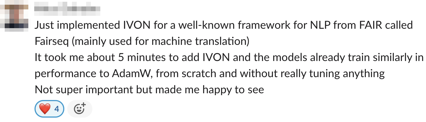
The team feels encouraged that their hard work is paying off. We are happy to receive feedback from the community about their experiences which we hope will be a pleasant one. Fingers crossed!

How do we use IVON to make predictions? The straightforward method is to simply use the $m$ vector of IVON like the trained weights $\theta$ in AdamW. For instance, we can simply do the following:

for X, y in test_loader:
    logit = model(X)
    _, prediction = logit.max(1)

A better way is to use “posterior averaging”. Essentially, we sample multiple $\theta$ from a Gaussian, make predictions using each $\theta$, and average the prediction to get the predictive probabilities. Below, is an example code for this.

for X, y in test_loader:
    sampled_probs = []
    for i in range(test_samples):
        with optimizer.sampled_params():
            sampled_logit = model(X)
            sampled_probs.append(F.softmax(sampled_logit, dim=1))
    prob = torch.mean(torch.stack(sampled_probs), dim=0)
    _, prediction = prob.max(1)

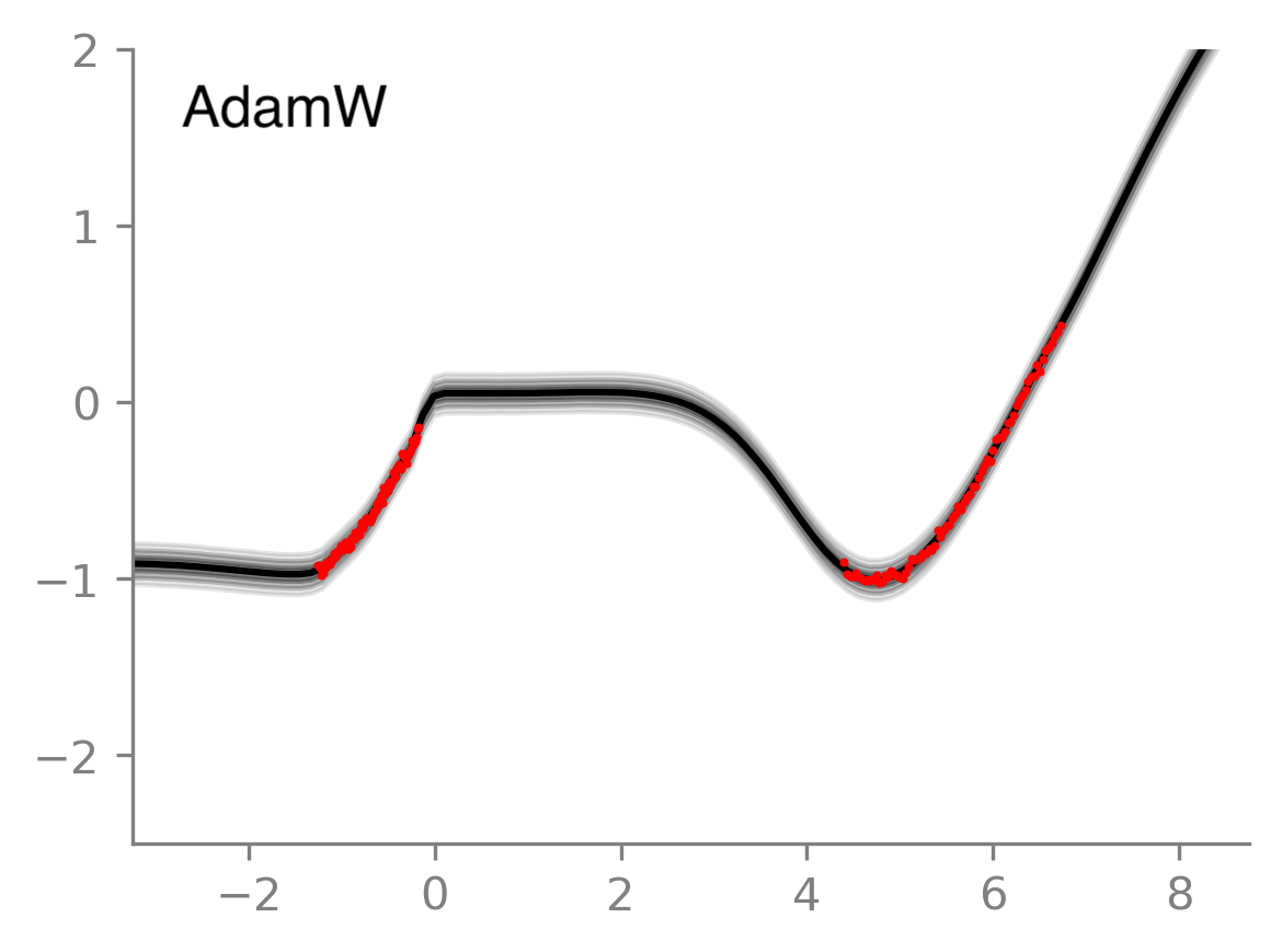
The second way gives us a way to compute confidence in the prediction. See this 1-D regression example in a Colab notebook, where IVON’s posterior averaging gives less confident predictions in regions where there is no data (red dots indicate data). This is indicated by the higher spread of gray regions around the average prediction (shown with black line). One could use the neural network’s output uncertainty from Adam to do the same thing but it does not give satisfactory uncertainty even for this simple 1-D example; see the below plot on the right.

A few such use cases are given in the github repo. Posterior averaging can be beneficial to get better performance, as shown in the figure below. The dashed line is obtained by using just the mean (the first method above) while the solid line is obtained by using posterior averaging (the second method). As the number of Monte-Carlo samples are increased both Accuracy and Negative Log-Likelihood (NLL) improve.

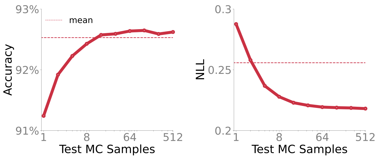
More samples give better estimate of the predictive probabilities, which do not affect accuracy much, but yield much better NLL. This is important when making risky decisions based on the model’s predictions. For instance, if a model predicts that the patient has cancer or not, it matters if the probability of that decision is 0.90 or 0.51. Decisions based on prob >0.5 are the same in both cases, but they are essentially random guess when probability is 0.51. Posterior averaging can be useful to distinguish such cases.

OTHER RESULTS: OOD DETECTION

We also have results on OOD detection to validate the quality of uncertainty estimates. We train on one dataset (call it in-domain) and try to predict another dataset that we believe to be different from the dataset (call it out-of-domain or OOD). We expect the predictions to generally be more confident on the in-domain dataset (smaller predictive entropy) and less confident on OOD dataset (larger predictive entropy). The figure below shows histograms of predictive entropies for a model trained on CIFAR-10 and tested for OOD on Flowers102. Look at SGD first: the histograms are skewed towards lower values no matter which dataset it is; red-ish colors are in-domain and gray-ish colors are OOD but they both have peaks at lower values. Now compare this to IVON, which has a high peak (indicated by dark red) at lower values for in-domain but generally assigns much higher values to OOD data (gray histogram is spread out to higher values). Overall, the difference between the OOD and in-domain histograms is more pronounced with IVON.

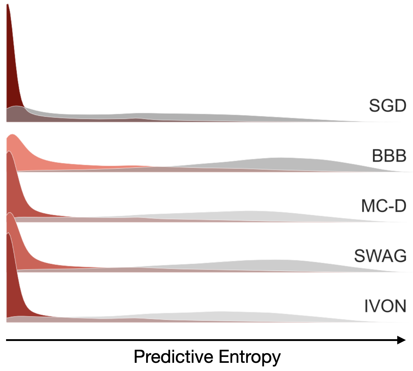
Other methods are somewhere in between, with BBB being the worst. For both SWAG and MC-Dropout the peak for in-domain is not as high. The results are not conclusive to outright reject these two methods but with IVON we are able to get reasonable results while directly optimizing the variational bounds. The result supports our hypothesis that variational learning can be effective at large scale.

OTHER RESULTS: MODEL MERGING IN LLMS

An attractive feature of IVON is that it yields, with no significant overhead, a sensible estimate of the second-order information $h$. This is essentially the inverse of $\sigma^2$ because $\sigma^2 = 1/(h+\delta)$. An estimate of $h$ is available throughout training and we can use it for knowledge transfer and understanding. Methods such as SGD, Adam, or SWAG require additional effort to estimate second-order information. I am also not aware of any other second-order optimizer that is as effective as IVON for deep learning. IVON is unique in this sense.

We show a use-case for model-merging in Large Language Models (LLM) where a recent practice is to merge many fine-tuned models by a simple arithmetic operation on their parameters. For example, given two fine-tuned models $\theta_1$ and $\theta_2$ using an LLM $\theta_{LLM}$, we can simply do the following,

\[\theta_{Merged} = \theta_{LLM} + (\theta_1 - \theta_{LLM}) + (\theta_2 - \theta_{LLM}).\]

This is called task arithmetic, but a better way is to rescale these estimates by Hessian vectors (here, for simplicity, we will use $h$ to denote $h+\delta$),

\[\theta_{Merged} = \theta_{LLM} + \frac{h_1}{h_1+h_2} \cdot (\theta_1 - \theta_{LLM}) + \frac{h_2}{h_1+h_2} \cdot (\theta_2 - \theta_{LLM}).\]

It is not hard to see why this is better. For example, the model with a large curvature (large $h$) should get a higher weight. In other words, the model with higher uncertainty (higher $\sigma$ or equivalently lower $h$) is less reliable and should be discounted. The second-order information helps us to incorporate this additional information, which also leads to a better model-merging strategy as shown by Daheim et al. 2024.

When training with SGD or AdamW, we need to make additional effort to compute $h$. Often, an additional pass through the whole dataset is needed. For very large models, the estimate can be ill-conditioned, that is, it can have very small entries. IVON does not have this problem where we have an unbiased estimator of Hessian, coupled with a moving average, a weight-decay parameter $\delta$, and a correction term that ensures $h$ to be non-negative throughout. The result below for model-merging shows that IVON can match the performance of other Hessian techniques while incurring no computational overhead at all (SG is a method that computes square-of-gradients after training using SGD or AdamW type of methods).

OTHER RESULTS: MODEL UNDERSTANDING

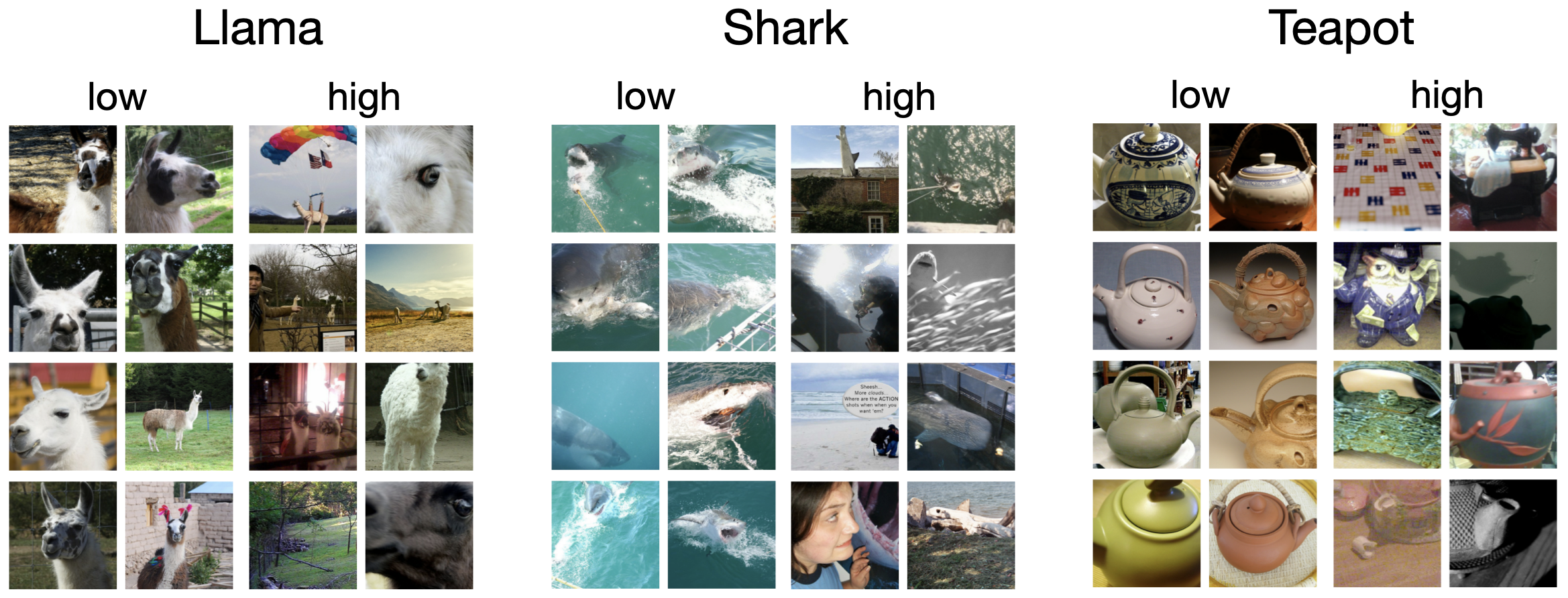
I will finish with a last result that is really exciting for me where we use $h$ to understand the dependence of the models on their training examples. Essentially, to estimate the importance of a set of examples, we can estimate how much the model would change when those examples are perturbed (for example, add or remove a subset of examples). In our recent work on memory-perturbation, we derived new techniques using the Bayesian learning rule. We show that, with IVON, we are able to estimate sensitivities during training and without a significant overhead. The calculations are simple and obtained as follows,

\[\text{sensitivity of an example} \propto \text{prediction error} \times \text{prediction variance}\]

I have omitted a constants here for simplicity, but the two quantities needed are readily available from IVON’s code, making estimation of sensitivity very easy. Below are some results on ImageNet where we see that low sensitivity examples conform to the categories they are assigned and high sensitivity examples are rather rebellious cases.

It is clear to me that second-order information is useful for such tasks. There are clear benefits to shift towards Newton-like methods. In my opinion, the advantage of second-order methods is not to just improve rates of convergence. Irrespective of that, there are plenty other uses of the second-order information. To appreciate this, it helps to think like a Bayesian. Posterior variance and second-order information are tightly connected, as it is clear from IVON’s pseudo-code. Therefore, any second-order method that improves Hessian estimation should also improve uncertainty estimates within a Bayesian framework. I strongly believe that optimization folks will benefit from these Bayesian insights.

A BRIEF HISTORY OF HOW WE GOT HERE

It has been a long journey for us to get here. I started this line of work way back in 2014 and published the first work on the Bayesian learning rule in 2017. The paper, although a personal breakthrough for me, focused on a narrow setting of variational inference and was difficult to appreciate for a broader audience. At the time, we wanted to build a codebase that would make the result more accessible to general machine-learning researchers. Fortunately or unfortunately, we decided to focus on deep learning instead and wrote a series of papers, specializing on Gaussian mean-field. These results were encouraging all along:

1. in our paper in 2018, we showed similarities to Adam;
2. in 2019, we matched the performance on ImageNet;
3. and in 2020, we solved the problem of difficult Hessian computation.

It was clear to me by this time that the algorithm should work, but I could not find a group of people who would push for a really good implementation that can be a drop-in replacement for SGD, Adam and similar methods. In 2021, Thomas Möllenhoff and colleagues did a simple implementation that won the NeurIPS 2021 challenge on Approximate Inference (you can check their presentation of the winning solution). This gave a good boost to the group to make some effort in developing a large-scale version.

We could have probably written a paper back then hastily, but we took 2 more years to make sure we do this well. Essentially, we had to find tricks that will work for most popular benchmarks and convince ourselves that this is really a good optimizer. Kudos to the team who made this a reality now! Thanks to Yuesong Shen (TU Munich) who continued to push through, to Nico Daheim (TU Darmstadt) for making the GPT-2 result a reality. Many thanks to their PhD supervisors as well. Thanks to Bai Cong and Clement Bazan for scaling the result to large models, and Rio Yokota for always supporting us with large-scale experiments. Thanks to Peter Nickl for doing the sensitivity experiments and Gian Maria Marconi for the RNN results and helping out with the competition. Most importantly, hats off to Thomas Möllenhoff for pushing this for 3 years, pushing on all front, helping all the members, and not giving up.

We find overwhelming evidence that IVON is a good optimizer, at least as good as any other optimizer that exists. For us, this is an important milestone because, we believe, IVON enables us to tackle the problem of knowledge understanding, transfer and collection. In coming years, we hope to have many new advances working towards an AI that can do continual lifelong learning just like we do. We hope that the community shares our enthusiasm and will also benefit from our work.